Plot SNIC imagery

Render image data processed by SNIC either from in-memory numeric arrays or from terra::SpatRaster objects provided by the terra package. The function supports plotting a single band or a three-channel RGB composite, with optional overlays for seed points and segmentation boundaries.

Usage

snic_plot(
  x,
  ...,
  band = 1L,
  r = NULL,
  g = NULL,
  b = NULL,
  col = getOption("snic.col", grDevices::hcl.colors(128L, "Spectral")),
  stretch = "lin",
  seeds = NULL,
  seeds_plot_args = getOption("snic.seeds_plot", list(pch = 20, col = "#00FFFF", cex =
    1)),
  seg = NULL,
  seg_plot_args = getOption("snic.seg_plot", list(border = "#FFD700", col = NA, lwd =
    0.6))
)

Arguments

x

Image data. For the array method this must be a numeric array with dimensions (height, width, bands). For the raster method the object must be a SpatRaster.

...

Additional arguments forwarded to the underlying plotting function. For arrays, these are passed to graphics::image(); for raster inputs they are forwarded to terra::snic_plot() (single band) or terra::plotRGB() (RGB composites).

band

Integer index of the band to display when producing a single-band plot. Defaults to the first band.

r, g, b

Integer indices (1-based) of the bands to use when composing an RGB plot. All three must be supplied to trigger RGB rendering and the image must contain at least three bands.

col

Color palette used for single-band plots. Ignored for RGB plots.

stretch

Character string indicating the contrast-stretching method. Determines how band values are scaled to the \([0, 1]\) range before plotting. One of:

• "lin": linear stretch based on the minimum and maximum values (default).

• "hist": histogram equalization (redistribute values to equalize the color histogram).

Non-numeric arrays or bands with only constant values are plotted as-is.

seeds

Optional object containing seed coordinates with columns r and c. Alternately, it can have SpatRaster inputs, lat and lon columns expressed in "EPSG:4326".

seeds_plot_args

Optional named list with additional arguments passed to graphics::points() when drawing seeds. Defaults to getOption("snic.seeds_plot"), falling back to list(pch = 16, col = "#00FFFF", cex = 1) which mirrors the internal .plot_seeds() defaults.

seg

For SpatRaster inputs, an optional segmentation raster (integer labels) or already vectorized segments (a terra::SpatVector) to be drawn over the image.

seg_plot_args

Named list of arguments forwarded to terra::snic_plot() for the seg overlay. The argument add = TRUE is set automatically when not supplied. Defaults to getOption("snic.seg_plot"), falling back to list(border = "#FFD700", col = NA, lwd = 0.6) which matches the defaults used inside .plot_segments().

Value

Invisibly, NULL.

Examples

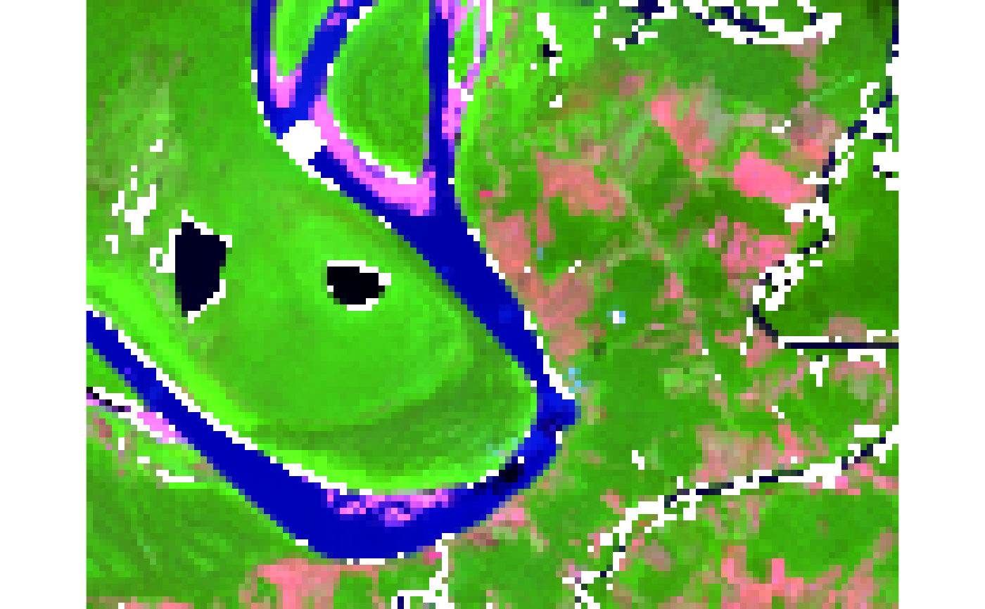
if (requireNamespace("terra", quietly = TRUE)) {
    tiff_dir <- system.file("demo-geotiff",
        package = "snic",
        mustWork = TRUE
    )
    files <- file.path(
        tiff_dir,
        c(
            "S2_20LMR_B02_20220630.tif",
            "S2_20LMR_B04_20220630.tif",
            "S2_20LMR_B08_20220630.tif",
            "S2_20LMR_B12_20220630.tif"
        )
    )

    # Load and optionally downsample for faster segmentation
    s2 <- terra::aggregate(terra::rast(files), fact = 8)

    # Visualize
    snic_plot(s2, r = 4, g = 3, b = 1, stretch = "lin")
}


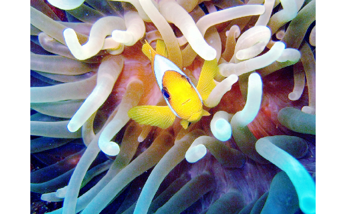
# Simple array example using bundled JPEG
if (requireNamespace("jpeg", quietly = TRUE)) {
    img_path <- system.file("demo-jpeg/clownfish.jpeg",
        package = "snic",
        mustWork = TRUE
    )

    # Load
    rgb <- jpeg::readJPEG(img_path)

    # Visualize
    snic_plot(rgb, r = 1, g = 2, b = 3, stretch = "none")
}