SNIC Segmentation Pipeline - SpatRaster

Introduction

This vignette revisits the SNIC segmentation pipeline, originally proposed by Achanta and Susstrunk (2017). It works with terra::SpatRaster objects, instead of a small in-memory RGB array. We will use the Sentinel-2 subset (demo-geotiff) that ships with the package. Every step reflects a typical remote-sensing workflow: load raster bands, seed the image, run snic(), and visualize the resulting segments.

Array workflow: If you prefer to start from in-memory arrays, see the SNIC Segmentation Pipeline - Arrays vignette for a compact tutorial that mirrors this tutorial without the geospatial dependencies.

Sentinel-2 preparation with terra

library(terra)

data_dir <- system.file("demo-geotiff", package = "snic", mustWork = TRUE)
band_files <- file.path(
  data_dir,
  c(
    "S2_20LMR_B02_20220630.tif",
    "S2_20LMR_B04_20220630.tif",
    "S2_20LMR_B08_20220630.tif",
    "S2_20LMR_B12_20220630.tif"
  )
)

s2 <- terra::rast(band_files)

names(s2) <- c("B02", "B04", "B08", "B12")
s2
#> class       : SpatRaster 
#> size        : 768, 1024, 4  (nrow, ncol, nlyr)
#> resolution  : 20, 20  (x, y)
#> extent      : 429960, 450440, 9046000, 9061360  (xmin, xmax, ymin, ymax)
#> coord. ref. : WGS 84 / UTM zone 20S (EPSG:32720) 
#> sources     : S2_20LMR_B02_20220630.tif  
#>               S2_20LMR_B04_20220630.tif  
#>               S2_20LMR_B08_20220630.tif  
#>               S2_20LMR_B12_20220630.tif  
#> names       : B02, B04, B08, B12

The four bands cover the blue (B02), red (B04), near-infrared (B08), and short-wave infrared (B12) portions of the spectrum. snic package comes with a helper function to plot false-color composites easily. snic_plot() understands both arrays and SpatRaster inputs.

snic_plot(s2, r = "B08", g = "B04", b = "B02")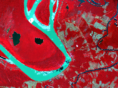

Figure 1 - A false-color composite of a Sentinel-2 scene.

Seeds creation

With a SpatRaster input, snic_grid() returns a data frame with latitude/longitude columns that can be inspected or stored for reproducibility.

seeds_rect <- snic_grid(s2, type = "rectangular", spacing = 24, padding = 2)

head(seeds_rect)
#>         lat       lon
#> 1 -8.491482 -63.63589
#> 2 -8.495824 -63.63590
#> 3 -8.500346 -63.63591
#> 4 -8.504688 -63.63592
#> 5 -8.509210 -63.63592
#> 6 -8.513733 -63.63593

spacing and padding parameters control the spacing (in pixels) between seeds and the padding (in pixels) around the image, respectively.

Run SNIC

The number of seeds controls the number of output segments. Seeds outside the image are ignored. The compactness parameter balances spatial proximity and spectral similarity; moderately low values emphasize spectral contrast, which is useful for multispectral imagery with distinct land-cover types. Here we use a compactness of 0.3.

seg_rect <- snic(s2, seeds_rect, compactness = 0.3)
seg_rect
#> SNIC segmentation
#>   Size (rows x cols):  768 x 1024
#> Viewing first rows and columns:
#> class       : SpatRaster 
#> size        : 6, 6, 1  (nrow, ncol, nlyr)
#> resolution  : 20, 20  (x, y)
#> extent      : 429960, 430080, 9061240, 9061360  (xmin, xmax, ymin, ymax)
#> coord. ref. : WGS 84 / UTM zone 20S (EPSG:32720) 
#> source(s)   : memory
#> name        : snic 
#> min value   :    1 
#> max value   :    1

The result is a snic object that contains a SpatRaster with same spatial extent as input but with one layer with integer labels. It also contains a data frame with per-segment feature means and centroids. The SpatRaster can be obtained by calling snic_get_seg(). The labels are 1-based and correspond to the seeds in the order they were provided.

Segments visualization

Here we plot the seed locations and the resulting segments on top of a false-color composite.

snic_plot(
  s2,
  r = "B08", g = "B04", b = "B02",
  stretch = "lin",
  seeds = seeds_rect,
  seeds_plot_args = list(pch = 3, col = "#00FFFF", cex = 0.6),
  seg = seg_rect,
  seg_plot_args = list(border = "#FFD700", col = NA, lwd = 0.5)
)

Figure 2 - The Sentinel-2 false-color composite with superpixel segmentation boundaries overlaid in yellow and seed points marked with cyan crosses.

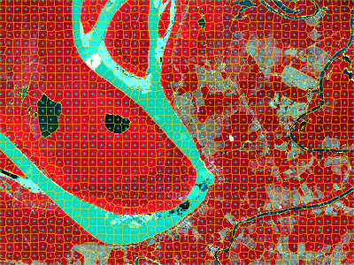
The segmentation result is a single-band SpatRaster whose values correspond to integer labels. You can extract statistics per segment or convert them to polygons via terra::as.polygons().

Comparative grid types and compactness values

All grid types available through snic_grid() operate on SpatRaster objects as well. Using the same Sentinel-2 subset, we compare rectangular, diamond, hexagonal, and random seeds combined with two compactness settings.

seeds_rect <- snic_grid(s2, type = "rectangular", spacing = 26)
seeds_diam <- snic_grid(s2, type = "diamond", spacing = 26)
seeds_hex  <- snic_grid(s2, type = "hexagonal", spacing = 26)

set.seed(42)
seeds_rand <- snic_grid(s2, type = "random", spacing = 26)

grids <- list(
  seeds_rect, seeds_diam,
  seeds_hex, seeds_rand
)

results <- lapply(grids, function(seeds) {
  list(
    snic(s2, seeds, compactness = 0.1),
    snic(s2, seeds, compactness = 0.4)
  )
})

op <- par(mfrow = c(4, 2), oma = c(2, 2, 2, 0))

for (res in results) {
  snic_plot(
    s2,
    r = "B08", g = "B04", b = "B02",
    seg = res[[1]],
    seg_plot_args = list(border = "#FFFFFF", col = NA, lwd = 0.4),
    mar = c(1, 0, 0, 0)
  )
  snic_plot(
    s2,
    r = "B08", g = "B04", b = "B02",
    stretch = "lin",
    seg = res[[2]],
    seg_plot_args = list(border = "#FFFFFF", col = NA, lwd = 0.4),
    mar = c(1, 0, 0, 0)
  )
}

mtext("Compactness = 0.1", side = 3, outer = TRUE, at = 0.25, line = 0.5)
mtext("Compactness = 0.4", side = 3, outer = TRUE, at = 0.75, line = 0.5)
mtext("Rectangular", side = 2, outer = TRUE, at = 3.5 / 4, line = 0.5, las = 3)
mtext("Diamond", side = 2, outer = TRUE, at = 2.5 / 4, line = 0.5, las = 3)
mtext("Hexagonal", side = 2, outer = TRUE, at = 1.5 / 4, line = 0.5, las = 3)
mtext("Random", side = 2, outer = TRUE, at = 0.5 / 4, line = 0.5, las = 3)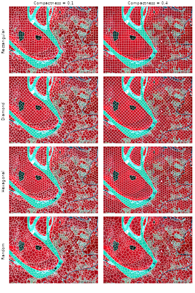

Figure 3 - Superpixel segmentation results on the Sentinel-2 scene. Rows correspond to different seed grid types (rectangular, diamond, hexagonal, random) and columns correspond to different compactness values (0.1 and 0.4).

par(op)

Rectangular and diamond layouts align segments with cardinal directions, whereas hexagonal and random seeds spread centers more evenly in all directions. Higher compactness induces smoother, more rounded superpixels, so the right column contains fewer jagged boundaries than the left one. Regardless of the seed geometry, the workflow stays the same: read the multi-band raster, place seeds in geographic space, and call snic() with the desired compactness.

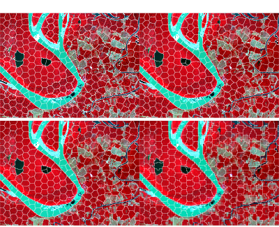
Fixed hexagonal seeds across resolutions

Spatial datasets often come in multiple resolutions—for example, you might start from a 10 m grid and also work with 20 m or 40 m aggregates for faster experimentation. Because snic_grid() returns seeds with geographic coordinates, the same seed set can be re-used across rasters that share the same extent and CRS. Below we generate a hexagonal grid once, then aggregate the Sentinel-2 raster to four different resolutions with terra::aggregate() and run snic() on each version without touching the seeds.

seeds_hex <- snic_grid(
  s2,
  type = "hexagonal",
  spacing = 50,
  padding = 5
)

The figure below compares the resulting segments.

op <- par(mfrow = c(2, 2), oma = c(0, 0, 2, 0))

agg_facts <- c(1L, 2L, 4L, 8L)
for (fact in agg_facts) {
  s2_agg <- terra::aggregate(s2, fact = fact, fun = "mean", na.rm = TRUE)
  seg_agg <- snic(s2_agg, seeds_hex, compactness = 0.2)
  snic_plot(
    s2_agg,
    r = "B08", g = "B04", b = "B02",
    seg = seg_agg,
    seg_plot_args = list(border = "white", col = NA, lwd = 0.4),
    main = sprintf("resolution %d m", fact * 20)
  )
}

Figure 4 - Superpixel segmentation results on the Sentinel-2 scene at different spatial resolutions (20 m, 40 m, 80 m, 160 m).

par(op)

References

Achanta, R., & Susstrunk, S. (2017). Superpixels and polygons using simple non-iterative clustering. Proceedings of the IEEE Conference on Computer Vision and Pattern Recognition (CVPR). doi:10.1109/CVPR.2017.520