SNIC Segmentation Pipeline - Arrays • snic

Introduction

The snic package implements the Simple Non-Iterative Clustering (SNIC) algorithm for image segmentation, originally proposed by Achanta and Susstrunk (2017). The objective of this tutorial is to present the segmentation pipeline in a compact, reproducible manner using a small example.

Remote sensing workflow: If you work with terra objects, see the SNIC Segmentation Pipeline - SpatRaster vignette for a step-by-step tutorial tailored to multispectral imagery.

Image preparation

if (!requireNamespace("jpeg", quietly = TRUE)) {
  stop("Install the 'jpeg' package to run this vignette.")
}

# Example RGB image shipped with the package (values in [0, 1])
img_path <- system.file("demo-jpeg/clownfish.jpeg", package = "snic",
  mustWork = TRUE)
rgb <- jpeg::readJPEG(img_path)
dim(rgb) # rows, cols, channels
#> [1]  900 1200    3

The rgb array is a 3-channel RGB image with dimensions 900 x 1200 pixels. R arrays are stored in column-major order, that means the contiguous memory layout stores pixels of a column before moving to the next column. Once all columns of a channel are stored, a new channel begins.

snic_plot(rgb, r = 1, g = 2, b = 3)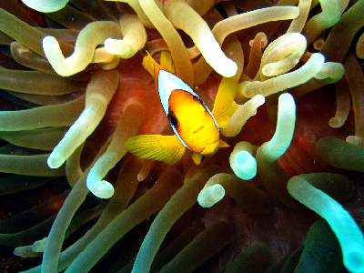

Figure 1 - An RGB image of a clownfish.

Lab color space

Achanta and Susstrunk (2017) use the Lab color space. To convert the RGB image to Lab, we use the convertColor() function from the grDevices package. First we have to reshape the image to a matrix with rows as image pixels and columns as color channels.

dims <- dim(rgb)
dim(rgb) <- c(dims[1] * dims[2], dims[3])

lab <- convertColor(rgb, from = "sRGB", to = "Lab", scale.out = 1 / 255)

# Back to canonical dimensions
dim(rgb) <- dims
dim(lab) <- dims

We can use the snic_plot() function to display the Lab image and visualize such transformations by comparing Lab channels with RGB channels as follows.


# Grayscale palette
gray <- grDevices::gray.colors(256)

# Prepare figure layout
op <- par(mfrow = c(2, 3))

# Plot Lab channels
snic_plot(lab, band = 1, col = gray, main = "L")
snic_plot(lab, band = 2, col = gray, main = "a")
snic_plot(lab, band = 3, col = gray, main = "b")

# Plot RGB channels
snic_plot(rgb, band = 1, col = gray, main = "R")
snic_plot(rgb, band = 2, col = gray, main = "G")
snic_plot(rgb, band = 3, col = gray, main = "B")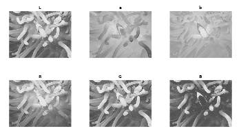

Figure 2 - Comparison of the L, a, b channels (Lab color space) with the R, G, B channels (RGB color space).


par(op)

The Lab transformation cannot be done if one want use multispectral images like satellite images, which have more than three channels and comprise of different wavelengths other than red, green and blue.

Once prepared the image to be segmented we can create seeds and run SNIC following the pipeline described below.

Seeds creation

Seeds are the initial cluster centers. The package provides a function to create seeds on a grid: snic_grid(). The function takes the image, the type of grid, and the spacing between seeds as arguments.

seeds <- snic_grid(lab, type = "rectangular", spacing = 22L)

The seeds are stored as data frame with columns r and c, representing the row and column indices of the seeds in the image.

The function supports four different types of grid: “rectangular”, “diamond”, “hexagonal”, and “random”. The spacing parameter controls the spacing between seeds. For random seeds, the spacing parameter means the expected spacing between seeds. The density of seeds is the inverse of the spacing.

Run SNIC

The number of seeds define the number of segments. The compactness parameter controls the trade-off between geometric distance and feature similarity. The greater the compactness, more weight is given to geometric distance between pixels, and less to feature similarity. The default value is 0.5.

segs <- snic(lab, seeds, compactness = 0.25)

Here, we defined a compactness of 0.25, which means that the algorithm will balance compactness and connectivity.

Segments visualization

snic_plot(rgb, r = 1, g = 2, b = 3, seg = segs)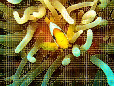

Figure 3 - The clownfish image with superpixel segmentation boundaries overlaid.

The variable segs is an array of the same dimensions as the input image, containing the segment labels for each pixel. It can be used to extract features from the image, or to apply other image processing operations.

dim(segs)
#> NULL

Now that we followed the entire pipeline, we can explore different grid types and compactness values to see how they affect the segmentation.

Comparative grid types and compactness values

We consider four seed arrangements generated by snic_grid(): rectangular, diamond, hexagonal, and random. All are built with the same expected spacing.


seeds_rect <- snic_grid(rgb, type = "rectangular", spacing = 22L)
seeds_diam <- snic_grid(rgb, type = "diamond", spacing = 22L)
seeds_hex  <- snic_grid(rgb, type = "hexagonal", spacing = 22L)

# Set seed for reproducibility
set.seed(42)
seeds_rand <- snic_grid(rgb, type = "random", spacing = 22L)

We expect that the density of seeds among the different grid types are similar given the same spacing. This may differ slightly due to geometrical boundary effects.

For comparison, we use two compactness values: 0.1 and 0.5.

grids <- list(
  seeds_rect, seeds_diam, seeds_hex, seeds_rand
)

results <- lapply(grids, function(seeds) {
  list(
    snic(rgb, seeds, compactness = 0.1),
    snic(rgb, seeds, compactness = 0.5)
  )
})

The panels below display the RGB image with superpixel boundaries overlaid for each grid type (rows) and compactness value (columns).


# Prepare figure layout
op <- par(mfrow = c(4, 2), oma = c(2, 2, 2, 0))

# Plot results
for (res in results) {
  snic_plot(rgb, r = 1, g = 2, b = 3, seg = res[[1]], mar = c(1, 0, 0, 0))
  snic_plot(rgb, r = 1, g = 2, b = 3, seg = res[[2]], mar = c(1, 0, 0, 0))
}

mtext("Compactness = 0.1", side = 3, outer = TRUE, at = 0.25, line = 0.5)
mtext("Compactness = 0.5", side = 3, outer = TRUE, at = 0.75, line = 0.5)
mtext("Rectangular", side = 2, outer = TRUE, at = 3.5 / 4, line = 0.5, las = 3)
mtext("Diamond", side = 2, outer = TRUE, at = 2.5 / 4, line = 0.5, las = 3)
mtext("Hexagonal", side = 2, outer = TRUE, at = 1.5 / 4, line = 0.5, las = 3)
mtext("Random", side = 2, outer = TRUE, at = 0.5 / 4, line = 0.5, las = 3)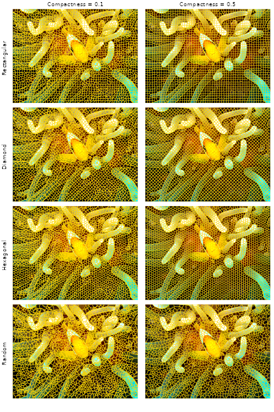

Figure 4 - Superpixel segmentation results on the clownfish image. Rows correspond to different seed grid types (rectangular, diamond, hexagonal, random) and columns to different compactness values (0.1 and 0.5).


par(op)

Under moderate to high compactness condition, the rectangular and diamond arrangements yield more axis-aligned boundary structure, while the hexagonal and randomized seeds distribute initial cluster centers more evenly in all directions. The choice among these layouts is task-dependent; the pipeline itself remains the same: define seeds, run snic(), and examine the resulting segments.

References

Achanta, R., & Susstrunk, S. (2017). Superpixels and polygons using simple non-iterative clustering. Proceedings of the IEEE Conference on Computer Vision and Pattern Recognition (CVPR). doi:10.1109/CVPR.2017.520