Spatial grid seeding for SNIC segmentation

Generate seed locations on an image following one of four spatial arrangements used in SNIC (Simple Non-Iterative Clustering) segmentation: rectangular, diamond, hexagonal, or random. Works for both numeric arrays and SpatRaster objects.

Usage

snic_grid(
  x,
  type = c("rectangular", "diamond", "hexagonal", "random"),
  spacing,
  padding = spacing/2,
  ...
)

snic_count_seeds(x, spacing, padding = spacing/2)

Arguments

x: Image data. For arrays, this must be numeric with dimensions (height, width, bands). For SpatRaster objects, raster dimensions are inferred automatically.
type: Character string indicating the spatial pattern to generate. One of "rectangular", "diamond", "hexagonal", or "random".
spacing: Numeric or integer. Either one value (applied to both axes) or two values (vertical, horizontal) giving the spacing between seeds in pixels.
padding: Numeric or integer. Distance from image borders within which no seeds are placed. May be of length 1 or 2. Defaults to spacing / 2.
...: Currently unused; reserved for future extensions.

Value

A data frame containing:

r, c when x has no CRS.
lat, lon when x has a CRS, expressed in EPSG:4326.

Details

The spacing parameter controls seed density. Padding shifts the seed grid inward so that seeds are not placed directly on image borders.

The spatial arrangements are:

rectangular: regular grid aligned with rows and columns.
diamond: alternating row offsets, forming a diamond layout.
hexagonal: alternating offsets approximating a hexagonal tiling.
random: uniform random placement with similar expected density.

The helper snic_count_seeds estimates how many seeds would be generated for a rectangular lattice with the given spacing and padding, without computing coordinates. For type = "diamond" or "hexagonal", the actual number of seeds will be up to roughly twice this estimate (minus boundary effects). For "random", the estimate corresponds to the expected density.

If x has a coordinate reference system, the returned data frame includes geographic coordinates (lat, lon) in EPSG:4326.

Examples

# Example 1: Geospatial raster
if (requireNamespace("terra", quietly = TRUE)) {
    # Load example multi-band image (Sentinel-2 subset) and downsample
    tiff_dir <- system.file("demo-geotiff",
        package = "snic",
        mustWork = TRUE
    )
    files <- file.path(tiff_dir, c(
        "S2_20LMR_B02_20220630.tif",
        "S2_20LMR_B04_20220630.tif",
        "S2_20LMR_B08_20220630.tif",
        "S2_20LMR_B12_20220630.tif"
    ))
    s2 <- terra::aggregate(terra::rast(files), fact = 8)

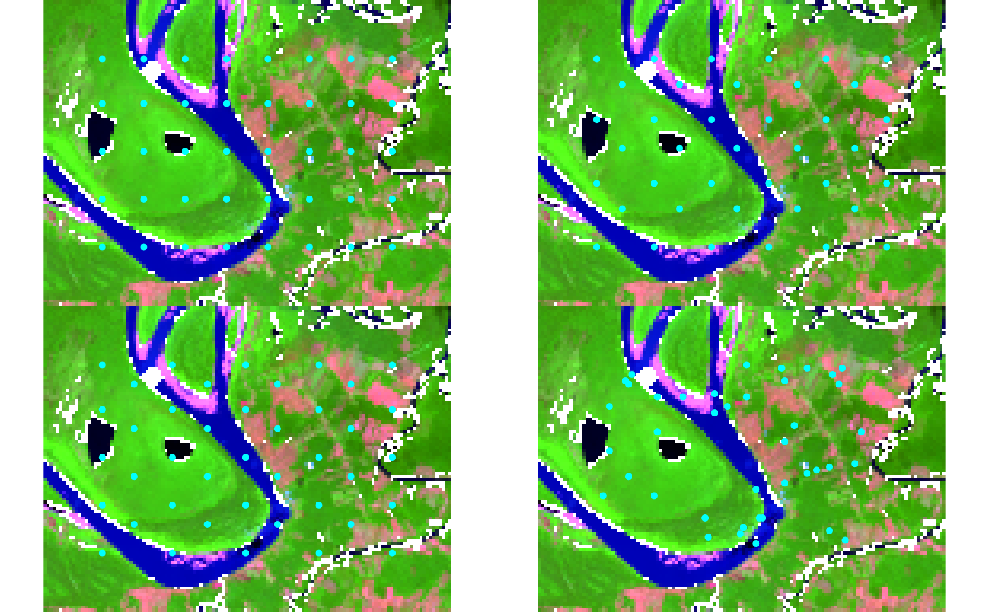
    # Compare grid types visually using snic_plot for immediate feedback
    types <- c("rectangular", "diamond", "hexagonal", "random")
    op <- par(mfrow = c(2, 2), mar = c(2, 2, 2, 2))
    for (tp in types) {
        seeds <- snic_grid(s2, type = tp, spacing = 12L, padding = 18L)
        snic_plot(
            s2,
            r = 4, g = 3, b = 1, stretch = "lin",
            seeds = seeds,
            main = paste("Grid:", tp)
        )
    }
    par(mfrow = c(1, 1))

    # Estimate seed counts for planning
    snic_count_seeds(s2, spacing = 12L, padding = 18L)
    par(op)
}


# Example 2: In-memory image (JPEG)
if (requireNamespace("jpeg", quietly = TRUE)) {
    img_path <- system.file(
        "demo-jpeg/clownfish.jpeg",
        package = "snic",
        mustWork = TRUE
    )
    rgb <- jpeg::readJPEG(img_path)

    # Compare grid types visually using snic_plot for immediate feedback
    types <- c("rectangular", "diamond", "hexagonal", "random")
    op <- par(mfrow = c(2, 2), mar = c(2, 2, 2, 2))
    for (tp in types) {
        seeds <- snic_grid(rgb, type = tp, spacing = 12L, padding = 18L)
        snic_plot(
            rgb,
            r = 1, g = 2, b = 3,
            seeds = seeds,
            main = paste("Grid:", tp)
        )
    }
    par(mfrow = c(1, 1))
    par(op)
}