Simple Non-Iterative Clustering (SNIC) segmentation

Segment an image into superpixels using the SNIC algorithm. This function wraps a C++ implementation operating on any number of spectral bands and uses 4-neighbor (von Neumann) connectivity.

Usage

snic(x, seeds, compactness = 0.5, ...)

Arguments

x

Image data. For the array method this must be a numeric array with dimensions (height, width, bands) in column-major order (R's native storage). For the SpatRaster method (from terra), dimensions and band ordering are inferred automatically.

seeds

Initial seed coordinates. The required format depends on the spatial status of x:

• If x has no CRS: a two-column data frame (r, c) giving 1-based pixel coordinates.

• If x has a CRS: a two-column data frame with columns lat and lon expressed in EPSG:4326. These are converted internally to pixel coordinates before segmentation.

Seeds define the starting cluster centers. They are usually generated with snic_grid helpers (e.g. rectangular, hexagonal or random), or placed interactively via snic_grid_manual.

compactness

Non-negative numeric value controlling the balance between feature similarity and spatial proximity (default = 0.5). Larger values produce more spatially compact superpixels.

...

Currently unused; reserved for future extensions.

Value

An object of class snic bundling the segmentation result together with per-cluster summaries produced by the SNIC algorithm. The segmentation result can be accessed using snic_get_seg. The per-cluster summaries can be accessed using snic_get_means and snic_get_centroids.

Details

The algorithm performs clustering in a joint space that includes the image's spectral dimensions and two spatial coordinates. Each seed initializes a region, and pixels are assigned based on the SNIC distance metric combining spectral similarity and spatial distance, weighted by compactness.

See also

snic_grid for seed generation, snic_grid_manual for interactive placement, snic_plot for visualizing results.

Examples

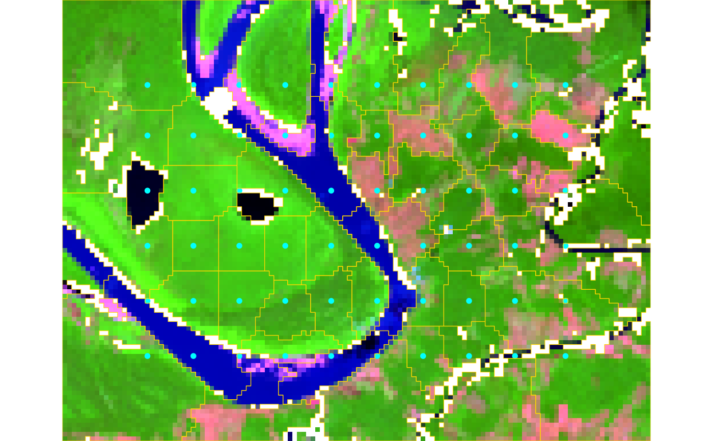
# Example 1: Geospatial raster
if (requireNamespace("terra", quietly = TRUE)) {
    path <- system.file("demo-geotiff", package = "snic", mustWork = TRUE)
    files <- file.path(
        path,
        c(
            "S2_20LMR_B02_20220630.tif",
            "S2_20LMR_B04_20220630.tif",
            "S2_20LMR_B08_20220630.tif",
            "S2_20LMR_B12_20220630.tif"
        )
    )

    # Downsample for speed (optional)
    s2 <- terra::aggregate(terra::rast(files), fact = 8)

    # Generate a regular grid of seeds (lat/lon because CRS is present)
    seeds <- snic_grid(
        s2,
        type    = "rectangular",
        spacing = 10L,
        padding = 18L
    )

    # Run segmentation
    seg <- snic(s2, seeds, compactness = 0.25)

    # Visualize RGB composite with seeds and segment boundaries
    snic_plot(
        s2,
        r = 4, g = 3, b = 1,
        stretch = "lin",
        seeds = seeds,
        seg = seg
    )
}


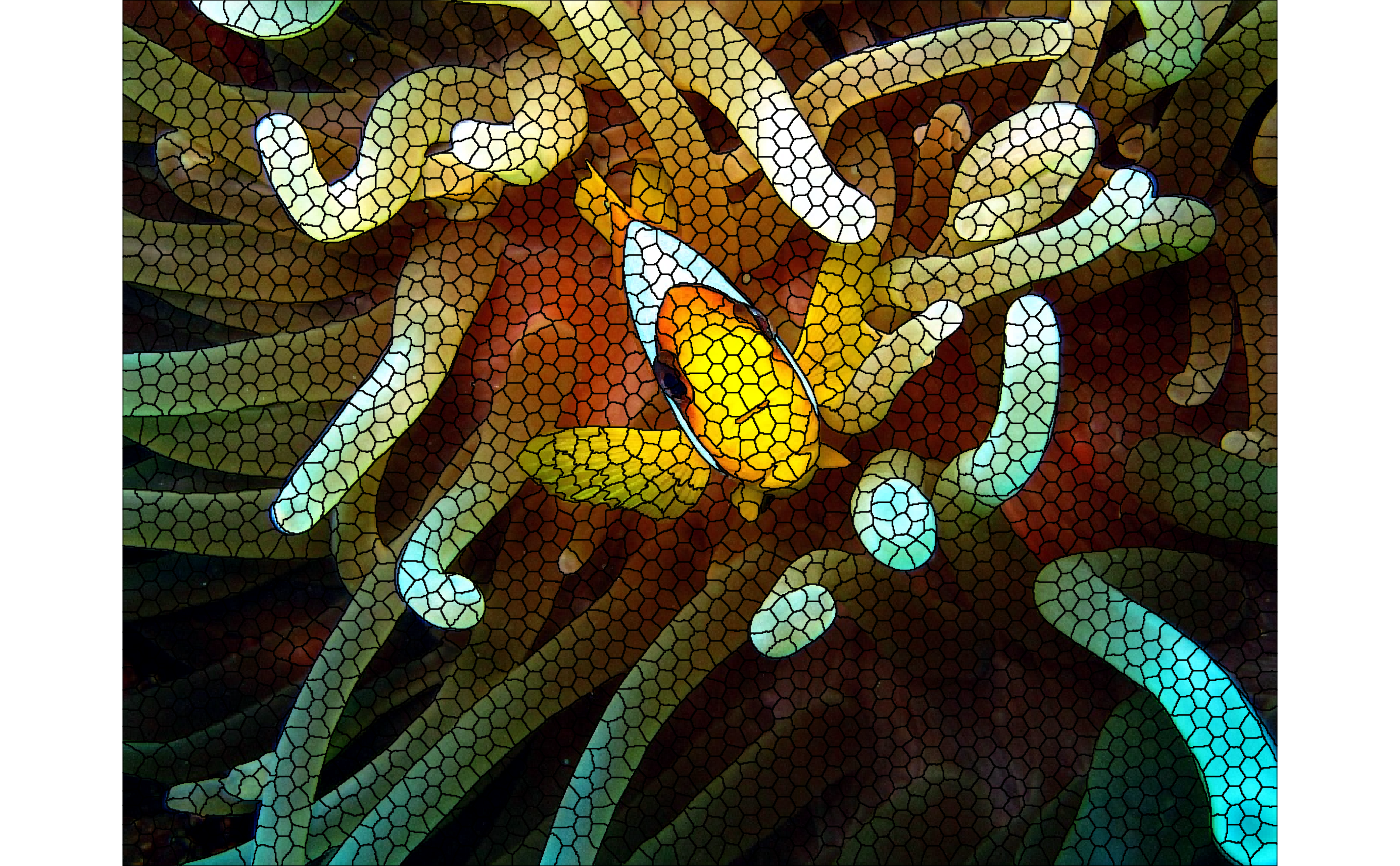
# Example 2: In-memory image (JPEG) + Lab transform
# Uses an example image shipped with the package (no terra needed)
if (requireNamespace("jpeg", quietly = TRUE)) {
    img_path <- system.file(
        "demo-jpeg/clownfish.jpeg",
        package = "snic",
        mustWork = TRUE
    )
    rgb <- jpeg::readJPEG(img_path) # h x w x 3 in [0, 1]

    # Convert sRGB -> CIE Lab for perceptual clustering
    dims <- dim(rgb)
    dim(rgb) <- c(dims[1] * dims[2], dims[3])
    lab <- grDevices::convertColor(
        rgb,
        from = "sRGB",
        to = "Lab",
        scale.in = 1,
        scale.out = 1 / 255
    )
    dim(lab) <- dims
    dim(rgb) <- dims

    # Seeds in pixel coordinates for array inputs
    seeds_rc <- snic_grid(lab, type = "hexagonal", spacing = 20L)

    # Segment in Lab space and plot L channel with boundaries
    seg <- snic(lab, seeds_rc, compactness = 0.1)

    snic_plot(
        rgb,
        r = 1L,
        g = 2L,
        b = 3L,
        seg = seg,
        seg_plot_args = list(
            border = "black"
        )
    )
}